Gene Set Similarity Tutorial
Rita M. Silva
2026-07-08
Source:vignettes/articles/Article_GeneSetSimilarity.Rmd
Article_GeneSetSimilarity.RmdEven if a user-defined gene signature demonstrates strong
discriminatory power between conditions, it may reflect known biological
pathways rather than novel mechanisms. To address this, the
geneset_similarity() function implements two complementary
similarity metrics:
Jaccard Index: the ratio of the number of genes in common over the total number of genes in the two sets.
Log Odds Ratio (logOR) from Fisher’s exact test of association between gene sets, given a specified gene universe.
Users can compare their signatures to:
-
Custom gene sets, defined manually;
-
MSigDB collections, via the
msigdbrpackage.
The function provides options to:
- Filter by Jaccard index threshold, using
jaccard_threshold; - Filter by odds ratio and p-value, using
or_thresholdandpval_threshold, respectively.
Similarity via Jaccard Index
The Jaccard index measures raw set overlap:
Example 1: Compare against user-defined and MSigDB gene sets
library(markeR)
#> Warning: markeR has been tested with ggplot2 <= 3.5.2. Using newer versions may cause incompatibilities.
# Example data
signature1 <- c("TP53", "BRCA1", "MYC", "EGFR", "CDK2")
signature2 <- c("ATXN2", "FUS", "MTOR", "CASP3")

signature_list <- list(
  "User_Apoptosis" = c("TP53", "CASP3", "BAX"),
  "User_CellCycle" = c("CDK2", "CDK4", "CCNB1", "MYC"),
  "User_DNARepair" = c("BRCA1", "RAD51", "ATM"),
  "User_MTOR" = c("MTOR", "AKT1", "RPS6KB1")
)

geneset_similarity(
  signatures = list(Sig1 = signature1, Sig2 = signature2),
  other_user_signatures = signature_list,
  collection = "C2",
  subcollection = "CP:KEGG_LEGACY",
  jaccard_threshold = 0.05,
  msig_subset = NULL,
  metric = "jaccard"
)$plot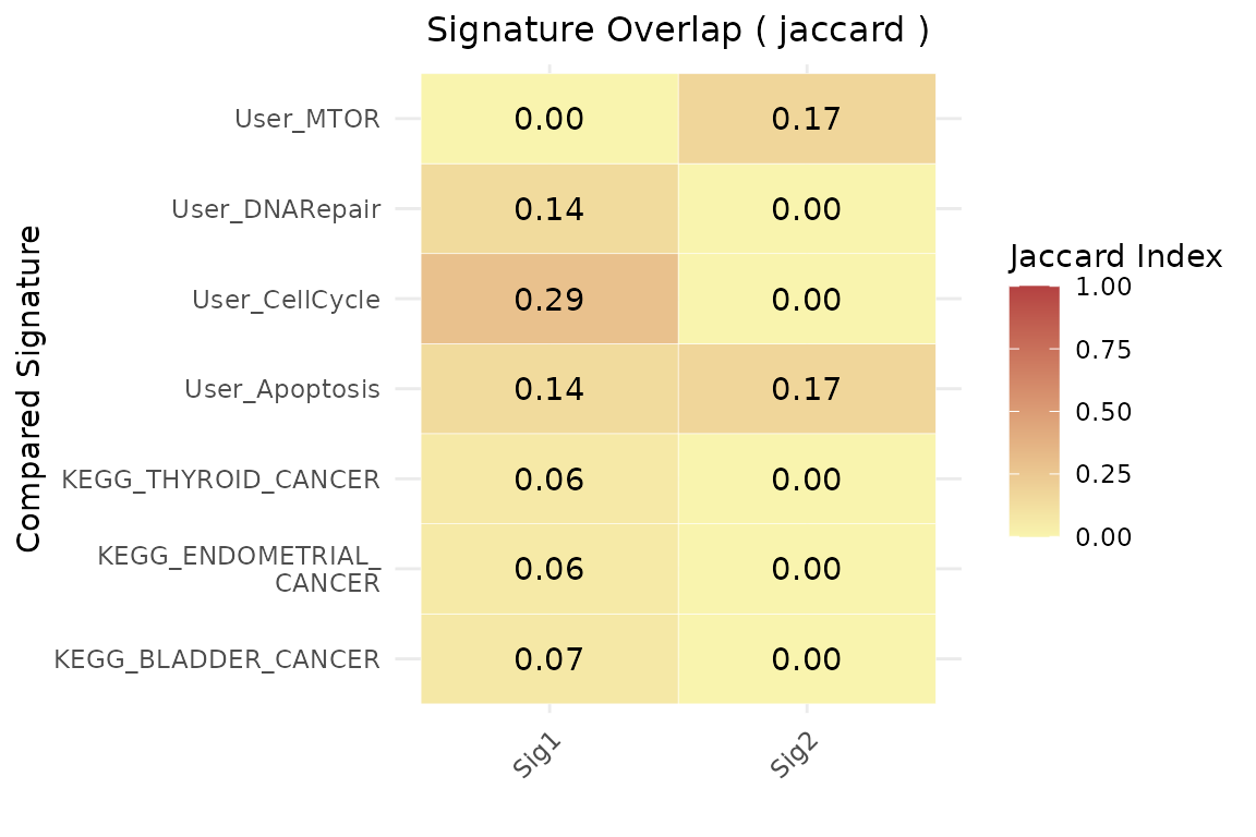
Example 2: Restrict comparison to a custom subset of MSigDB
geneset_similarity(
  signatures = list(Sig1 = signature1, Sig2 = signature2),
  other_user_signatures = NULL,
  collection = "C2",
  subcollection = "CP:KEGG_LEGACY",
  jaccard_threshold = 0,
  msig_subset = c("KEGG_MTOR_SIGNALING_PATHWAY", "KEGG_APOPTOSIS", "NON_EXISTENT_PATHWAY"),
  metric = "jaccard",
  limits=c(0,0.1)
)$plot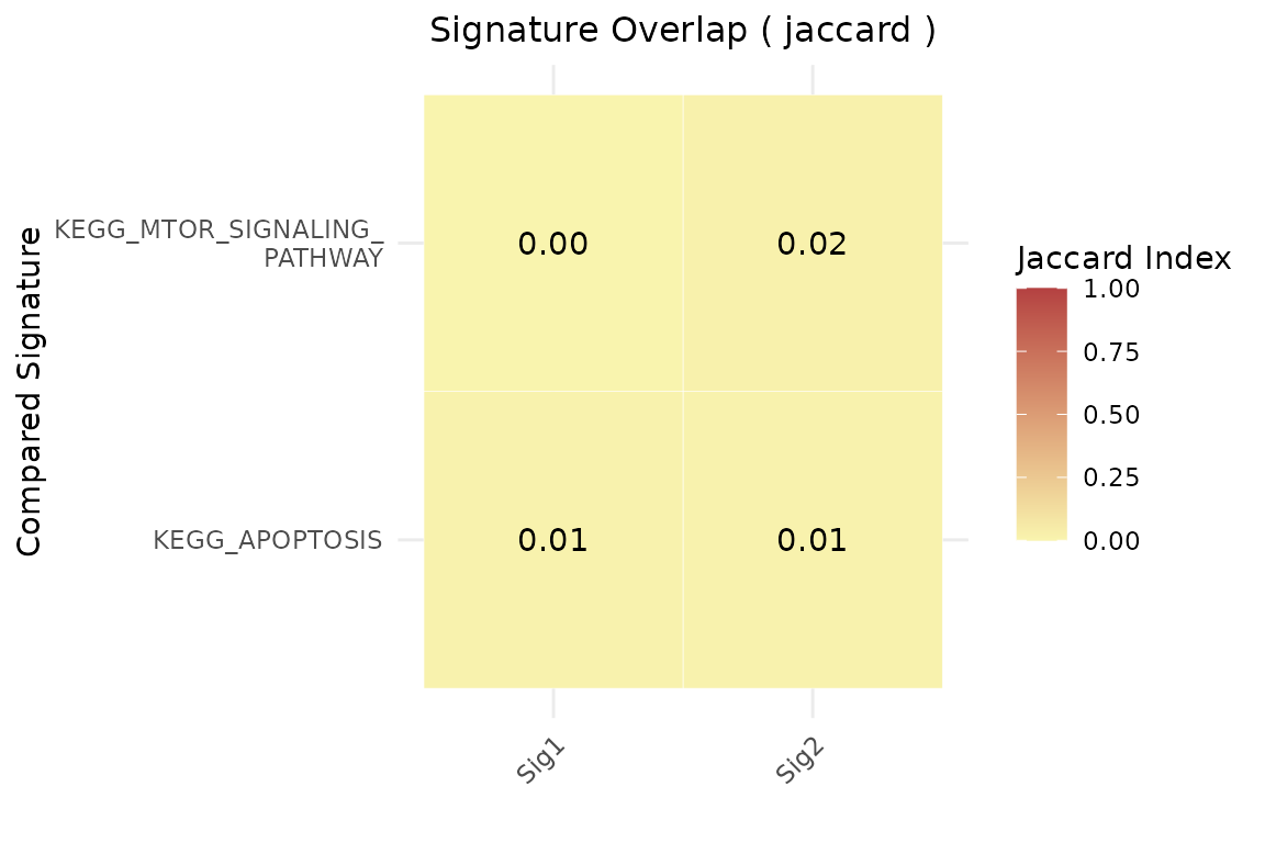
Similarity via Log Odds Ratio
The log odds ratio (logOR) provides a statistically grounded alternative for assessing gene set similarity. It measures enrichment of one set within another, relative to a defined background or gene universe, using a 2×2 contingency table.
-
Log odds ratio (logOR):
Derived from contingency tables using:- Genes in both sets
- Genes in one but not the other
- Gene universe as background
Note: When using
metric = "odds_ratio", theuniverseparameter must be supplied.
Example 3: Compare against user-defined and MSigDB gene sets
geneset_similarity(
  signatures = list(Sig1 = signature1, Sig2 = signature2),
  other_user_signatures = signature_list,
  collection = "C2",
  subcollection = "CP:KEGG_LEGACY",
  metric = "odds_ratio",
  # Define gene universe (e.g., genes from HPA or your dataset)
  universe = unique(c(
    signature1, signature2,
    unlist(signature_list),
    msigdbr::msigdbr(species = "Homo sapiens", category = "C2")$gene_symbol
  )),
  or_threshold = 100, #log10OR = 2
  width_text=50,
  pval_threshold = 0.05
)$plot
#> Warning: The `category` argument of `msigdbr()` is deprecated as of msigdbr 10.0.0.
#> ℹ Please use the `collection` argument instead.
#> This warning is displayed once per session.
#> Call `lifecycle::last_lifecycle_warnings()` to see where this warning was
#> generated.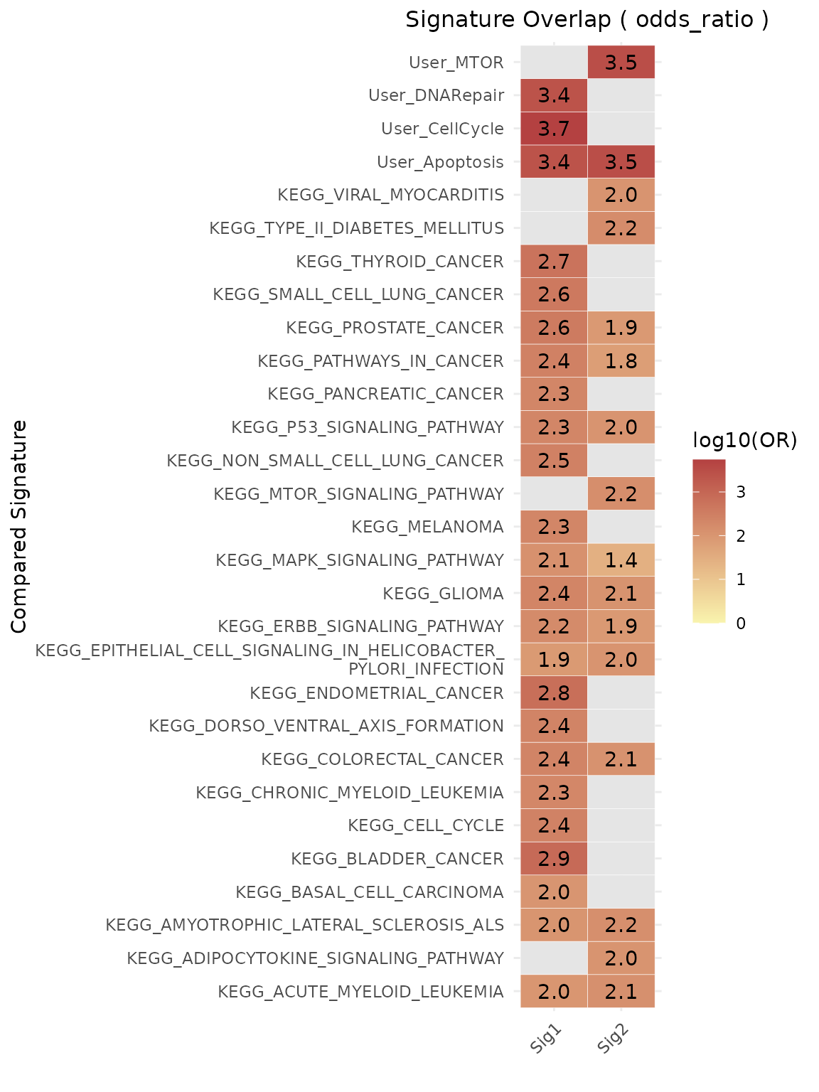
Session Information
sessionInfo()
#> R version 4.6.1 (2026-06-24)
#> Platform: x86_64-pc-linux-gnu
#> Running under: Ubuntu 24.04.4 LTS
#>
#> Matrix products: default
#> BLAS:   /usr/lib/x86_64-linux-gnu/openblas-pthread/libblas.so.3
#> LAPACK: /usr/lib/x86_64-linux-gnu/openblas-pthread/libopenblasp-r0.3.26.so;  LAPACK version 3.12.0
#>
#> locale:
#>  [1] LC_CTYPE=C.UTF-8       LC_NUMERIC=C           LC_TIME=C.UTF-8
#>  [4] LC_COLLATE=C.UTF-8     LC_MONETARY=C.UTF-8    LC_MESSAGES=C.UTF-8
#>  [7] LC_PAPER=C.UTF-8       LC_NAME=C              LC_ADDRESS=C
#> [10] LC_TELEPHONE=C         LC_MEASUREMENT=C.UTF-8 LC_IDENTIFICATION=C
#>
#> time zone: UTC
#> tzcode source: system (glibc)
#>
#> attached base packages:
#> [1] stats     graphics  grDevices utils     datasets  methods   base
#>
#> other attached packages:
#> [1] markeR_1.3.1
#>
#> loaded via a namespace (and not attached):
#>   [1] pROC_1.19.0.1         gridExtra_2.3.1       rlang_1.3.0
#>   [4] magrittr_2.0.5        clue_0.3-68           GetoptLong_1.1.1
#>   [7] msigdbr_26.1.0        otel_0.2.0            matrixStats_1.5.0
#>  [10] compiler_4.6.1        png_0.1-9             systemfonts_1.3.2
#>  [13] vctrs_0.7.3           reshape2_1.4.5        stringr_1.6.0
#>  [16] pkgconfig_2.0.3       shape_1.4.6.1         crayon_1.5.3
#>  [19] fastmap_1.2.0         backports_1.5.1       labeling_0.4.3
#>  [22] effectsize_1.0.3      rmarkdown_2.31        ragg_1.5.2
#>  [25] purrr_1.2.2           xfun_0.59             cachem_1.1.0
#>  [28] jsonlite_2.0.0        BiocParallel_1.46.0   broom_1.0.13
#>  [31] parallel_4.6.1        cluster_2.1.8.2       R6_2.6.1
#>  [34] stringi_1.8.7         bslib_0.11.0          RColorBrewer_1.1-3
#>  [37] limma_3.68.4          car_3.1-5             jquerylib_0.1.4
#>  [40] Rcpp_1.1.2            assertthat_0.2.1      iterators_1.0.14
#>  [43] knitr_1.51            parameters_0.29.2     IRanges_2.46.0
#>  [46] Matrix_1.7-5          tidyselect_1.2.1      abind_1.4-8
#>  [49] yaml_2.3.12           doParallel_1.0.17     codetools_0.2-20
#>  [52] curl_7.1.0            plyr_1.8.9            lattice_0.22-9
#>  [55] tibble_3.3.1          withr_3.0.3           bayestestR_0.18.1
#>  [58] S7_0.2.2              evaluate_1.0.5        desc_1.4.3
#>  [61] circlize_0.4.18       pillar_1.11.1         ggpubr_1.0.0
#>  [64] carData_3.0-6         foreach_1.5.2         stats4_4.6.1
#>  [67] insight_1.5.2         generics_0.1.4        S4Vectors_0.50.1
#>  [70] ggplot2_4.0.3         scales_1.4.0          glue_1.8.1
#>  [73] tools_4.6.1           data.table_1.18.4     fgsea_1.38.0
#>  [76] locfit_1.5-9.12       ggsignif_0.6.4        babelgene_22.9
#>  [79] fs_2.1.0              fastmatch_1.1-8       cowplot_1.2.0
#>  [82] grid_4.6.1            tidyr_1.3.2           datawizard_1.3.1
#>  [85] edgeR_4.10.1          colorspace_2.1-2      Formula_1.2-5
#>  [88] cli_3.6.6             textshaping_1.0.5     ComplexHeatmap_2.28.0
#>  [91] dplyr_1.2.1           gtable_0.3.6          ggh4x_0.3.1
#>  [94] rstatix_1.0.0         sass_0.4.10           digest_0.6.39
#>  [97] BiocGenerics_0.58.1   ggrepel_0.9.8         rjson_0.2.23
#> [100] htmlwidgets_1.6.4     farver_2.1.2          htmltools_0.5.9
#> [103] pkgdown_2.2.1         lifecycle_1.0.5       GlobalOptions_0.1.4
#> [106] statmod_1.5.2