Introduction
markeR is an R package that provides a
modular and extensible framework for the systematic evaluation of gene
sets as phenotypic markers using transcriptomic data. The package is
designed to support both quantitative analyses and visual exploration of
gene set behaviour across experimental and clinical phenotypes.
In this vignette, we demonstrate the core functionalities of
markeR using a pre-processed gene expression dataset and
associated metadata from Marthandan et al. (2016) (GSE63577). This
dataset comprises human fibroblast samples cultured under two
experimental conditions: replicative senescence and proliferative
control.
Primary Objectives
The primary objectives of markeR are
to:
- Establish a reproducible and standardised framework for quantifying gene sets as phenotypic markers across transcriptomic datasets.
- Provide a unified interface for complementary analytical strategies, including score-based and enrichment-based methods.
- Enable systematic comparison of user-defined gene sets with curated reference collections (e.g., MSigDB) to enhance biological interpretability.
- Deliver modular tools for visualisation and evaluation, allowing exploration of both gene set behaviour and individual gene-level contributions.
Features and Capabilities
The package integrates multiple analytical strategies for quantifying phenotypes using gene sets, supporting both unidirectional and bidirectional (i.e., respectively without and with information on the expected direction of change in expression of genes upon phenotype) gene set definitions:
- Score-based methods: log2-median expression, ranking approaches, and single-sample gene set enrichment analysis (ssGSEA) to quantify coordinated expression within a gene set.
- Enrichment-based methods: GSEA using moderated t- or B-statistics.
- Gene-level exploration: expression heatmaps, violin plots, ROC curve analysis, area under the curve (AUC) calculations, effect size estimation, and principal component analysis (PCA) to characterise the contribution of individual genes.
- Gene set similarity assessment: Jaccard index and log odds ratio (logOR) calculations to compare user-defined gene sets with reference or user-defined collections.
The package is implemented with flexibility and extensibility as core
design principles. Visualisation leverages ggplot2,
ComplexHeatmap, ggpubr, cowplot,
and grid, enabling a wide range of customisation options.
The modular structure ensures compatibility with additional methods in
future versions of the package.
Installation
Install the latest release from Bioconductor:
# Install from Bioconductor
if (!requireNamespace("BiocManager", quietly = TRUE))
  install.packages("BiocManager")
BiocManager::install("markeR")
Or install the latest development release of markeR from
GitHub with:
devtools::install_github("DiseaseTranscriptomicsLab/markeR@*release")Common Workflow
Input Requirements
Gene Sets
A named list where each element is a gene set.
- Use a character vector when putative direction of change in expression of genes upon phenotype is unknown (unidirectional).
- Use a data frame with columns
geneanddirection(values+1for up-,-1for down-regulation) when direction is known (bidirectional).
# Example
gene_sets
## $Set1
## [1] "GeneA" "GeneB" "GeneC" "GeneD"
##
## $Set2
## gene direction
## 1 GeneX 1
## 2 GeneY -1
## 3 GeneZ 1For this vignette, we will use three senescence-related gene sets
that ship with the package (see ?genesets_example for more
information):
- LiteratureMarkers (bidirectional; gene set of commonly reported senescence markers in the literature)
- REACTOME_CELLULAR_SENESCENCE (unidirectional; from the MSigDB database)
- HernandezSegura (bidirectional; from Hernandez-Segura et al. (2017))
# Load example gene sets
data(genesets_example)
Expression Data Frame
A filtered and normalised, non log-transformed, gene expression matrix (genes × samples). Row names must be gene identifiers; column names must match sample IDs in the metadata.
Warning: If you are using microarray data or outputs
from common RNA-seq pipelines (e.g., edgeR), note that the
expression values may already be log2-normalised. The input to
markeR must necessarily be
non-log-transformed. If your data are log2-transformed,
you can revert them by applying 2^data.
In this vignette, we use a pre‑processed RNA-seq dataset from
Marthandan et al. (2016, GSE63577), with normalised read counts for
human fibroblasts under replicative senescence and
proliferative control. See ?counts_example
for structure.
# Load example expression data
data(counts_example)
counts_example[1:5, 1:5]
## SRR1660534 SRR1660535 SRR1660536 SRR1660537 SRR1660538
## A1BG 9.94566 9.476768 8.229231 8.515083 7.806479
## A1BG-AS1 12.08655 11.550303 12.283976 7.580694 7.312666
## A2M 77.50289 56.612839 58.860268 8.997624 6.981857
## A4GALT 14.74183 15.226083 14.815891 14.675780 15.222488
## AAAS 47.92755 46.292377 43.965972 47.109493 47.213739Sample Metadata
A data frame with samples as rows and annotations as columns. The first column should contain sample IDs matching the expression matrix column names.
We use the accompanying metadata from the Marthandan et al. (2016)
study. See ?metadata_example.
##       sampleID      DatasetID   CellType     Condition       SenescentType
## 252 SRR1660534 Marthandan2016 Fibroblast     Senescent Telomere shortening
## 253 SRR1660535 Marthandan2016 Fibroblast     Senescent Telomere shortening
## 254 SRR1660536 Marthandan2016 Fibroblast     Senescent Telomere shortening
## 255 SRR1660537 Marthandan2016 Fibroblast Proliferative                none
## 256 SRR1660538 Marthandan2016 Fibroblast Proliferative                none
## 257 SRR1660539 Marthandan2016 Fibroblast Proliferative                none
##                         Treatment
## 252 PD72 (Replicative senescence)
## 253 PD72 (Replicative senescence)
## 254 PD72 (Replicative senescence)
## 255                         young
## 256                         young
## 257                         young
Select Mode of Analysis
markeR provides two modes of operation:
Benchmarking: evaluates gene sets’ performance in marking a metadata variable, i.e., a phenotype, returning comparative visualisations across scoring and enrichment methods.
Discovery: examines the relationship between a gene set and one or more variables of interest, suitable for exploratory or hypothesis-generating analyses.
Choose a Quantification Approach
Two complementary strategies are implemented for quantifying associations between gene sets and phenotypes:
Score-Based Approach
A score summarising the collective expression of a gene set therein is assigned to each sample. Scores can be visualised using built-in functions, or used directly in downstream analyses (e.g., comparisons between phenotypic groups of samples, correlations with numerical phenotypes).
Available methods:
Log2-median: mean of the across-sample normalised log2 median-centred expression levels of the genes in the set; for bidirectional gene sets, the sample score is the partial score for the subset of putatively upregulated genes minus that of the downregulated subset.
Ranking: mean expression rank of gene set members in each sample; for bidirectional gene sets, the sample score is the partial score for the subset of putatively upregulated genes minus that of the downregulated subset, and normalised by the number of genes in the set.
ssGSEA: single-sample gene set enrichment score using ssGSEA; for bidirectional gene sets, the sample score is the partial score for the subset of putatively upregulated genes minus that of the downregulated subset.
Gene sets that are robust phenotypic markers are expected to yield consistently high scores across methods.
Enrichment-Based Approach
Enrichment-based methods implement Gene Set Enrichment Analysis (GSEA). Genes are ranked according to differential expression statistics, and a Normalised Enrichment Score (NES) per variable of interest is computed, accompanied by a p-value adjusted for multiple hypothesis testing.
Visualisation and Evaluation
Benchmarking Mode
markeR offers a range of visual summaries for
Benchmarking:
- Violin plots of score distributions by categorical phenotype;
- Scatter plots of association between scores and numerical phenotypes;
- Volcano plots and heatmaps of scores or differential gene set expression based on effect sizes (Cohen’s d or f);
- ROC curves and respective AUC values of gene sets’ phenotypic classification performance;
- Violin plots of effect size distributions (Cohen’s d) for pairwise group differences in scores, for original and simulated gene sets;
- Plots summarising NES alongside adjusted p-values (e.g., lollipop plots);
- GSEA plots showing running enrichment scores across ranked gene lists.
Example of common workflows in Benchmarking Mode (full tutorial here):
Score-based approaches
Score-based methods facilitate direct comparisons of gene set activity between phenotypic groups (e.g., being senescent) and can be used in downstream analyses, including for example correlation with other metadata variables of interest (e.g., day of sequencing) . We first compute log2-median scores. In this dataset, the HernandezSegura and LiteratureMarkers gene sets yield large effect sizes (|Cohen’s d|), whereas REACTOME_CELLULAR_SENESCENCE shows more modest separation between senescent and proliferative fibroblasts.
# Quantification approach: scores
# Method: log2-median
PlotScores(data = counts_example,
           metadata = metadata_example,
           gene_sets = genesets_example,
           Variable="Condition",
           method ="logmedian",
           nrow = 1,
           pointSize=4,
           title="Marthandan et al. 2016",
           widthTitle = 24,
           labsize=12,
titlesize = 12) 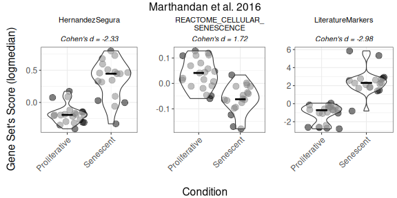
Next, scores are calculated using multiple methods (log2-median, ranking, ssGSEA) to assess consistency across strategies. Outputs include heatmaps and volcano plots of effect sizes (|Cohen’s d|). HernandezSegura and LiteratureMarkers consistently discriminate Senescent from Proliferative samples, while REACTOME_CELLULAR_SENESCENCE shows weaker and less consistent separation.
Overall_Scores <- PlotScores(data = counts_example,
                             metadata = metadata_example,
                             gene_sets=genesets_example,
                             Variable="Condition",
                             method ="all",
                             ncol = NULL,
                             nrow = 1,
                             widthTitle=30,
                             limits = c(0,3.5),
                             title="Marthandan et al. 2016",
                             titlesize = 10,
                             ColorValues = list(heatmap=c("#F9F4AE", "#B44141"),
                                                volcano=signature_colors <- c(
                                                  HernandezSegura = "#A07395",
                                                  REACTOME_CELLULAR_SENESCENCE = "#6B8E9E",
                                                  LiteratureMarkers = "#CA7E45"
                                                )
                             ),
                             mode="simple",
                             widthlegend=30,
                             sig_threshold=0.05,
                             cohen_threshold=0.6,
                             pointSize=6,
                             colorPalette="Paired")
Overall_Scores$heatmap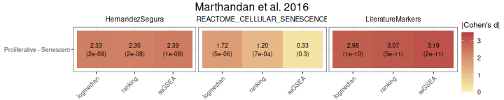
Overall_Scores$volcano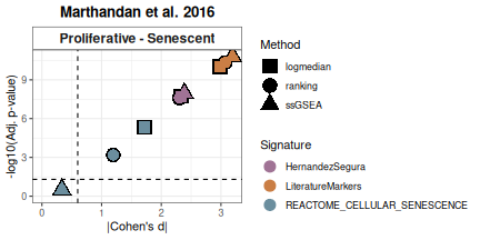
The discriminatory capacity of gene set scores can also be assessed using ROC curves and corresponding AUC values. HernandezSegura and LiteratureMarkers exhibit consistently high AUCs across scoring methods, while REACTOME_CELLULAR_SENESCENCE shows more heterogeneous performance.
ROC_Scores(data = counts_example,
           metadata = metadata_example,
           gene_sets=genesets_example,
           method = "all",
           variable ="Condition",
           colors = c(logmedian = "#3E5587", ssGSEA = "#B65285", ranking = "#B68C52"),
           grid = TRUE,
           spacing_annotation=0.3,
           ncol=NULL,
           nrow=1,
           mode = "simple",
           widthTitle = 28,
           titlesize = 10,
title="Marthandan et al. 2016") 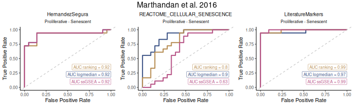
Finally, false positive rates for effect sizes are estimated by simulating random gene sets of equal size. This step provides a null distribution against which observed scores can be compared. In this example, the LiteratureMarkers signature demonstrates the strongest performance. Increasing the number of simulations would yield finer resolution at the cost of additional computational time.
set.seed("123456")
FPR_Simulation(data = counts_example,
               metadata = metadata_example,
               original_signatures = genesets_example,
               gene_list = row.names(counts_example),
               number_of_sims = 100,
               title = "Marthandan et al. 2016",
               widthTitle = 30,
               Variable = "Condition",
               titlesize = 12,
               pointSize = 5,
               labsize = 10,
               mode = "simple",
               ColorValues=NULL,
               ncol=NULL,
nrow=1 ) 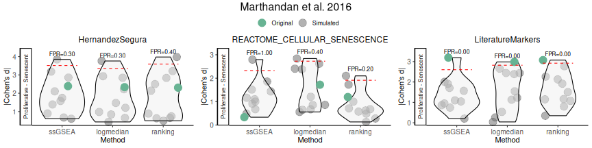
Enrichment-based approaches
The first step is the quantification of differential expression.
Here, a design matrix (as defined by the limma package) is
automatically constructed from the Condition variable in
the metadata, defining the contrast
Senescent - Proliferative. Internally, this fits a linear
model without an intercept, enabling quick comparison between levels of
a categorical variable.
# Build design matrix from variables (Condition) and apply a contrast.
# The design matrix is constructed automatically using the variable "Condition".
DEGs <- calculateDE(data = counts_example,
                    metadata = metadata_example,
                    variables = "Condition",
                    contrasts = c("Senescent - Proliferative"))
DEGs$`Senescent-Proliferative`[1:5,]
## logFC AveExpr t P.Value adj.P.Val B
## CCND2 3.816674 4.406721 12.379571 2.944841e-15 2.349757e-12 24.64395
## MKI67 -3.581174 6.605339 -9.187514 2.110510e-11 4.769568e-10 15.91258
## PTCHD4 3.398914 3.556007 10.729126 2.461327e-13 2.868691e-11 20.30116
## KIF20A -3.365481 5.934893 -9.718104 4.406643e-12 1.771710e-10 17.45858
## CDC20 -3.304602 6.104079 -9.791031 3.562991e-12 1.592176e-10 17.66821Differential expression results can be visualised with volcano plots. These highlight the magnitude of expression changes (log2 fold change) against statistical significance (adjusted p-value for the moderated t-statistic), with genes from predefined sets emphasised (up- in green and downregulated in red). In this example:
- Genes in the HernandezSegura set annotated as upregulated (green) display positive log2 fold changes, whereas those annotated as downregulated (red) show negative log2 fold changes. This pattern is consistent with the annotation of the set, although these genes are not necessarily those exhibiting the largest absolute fold changes.
- In the LiteratureMarkers set, LMNB1 and MKI67 exhibit strongly negative log2 fold change, consistent with their roles as proliferation markers absent in senescent cells.
- Genes from the REACTOME_CELLULAR_SENESCENCE set are undirected and appear across the full range of log2 fold change values, diluting discriminatory power.
# Change order: gene sets in columns, contrast in rows
plotVolcano(DEGs, genes = genesets_example,
            N = NULL,
            x = "logFC", y = "-log10(adj.P.Val)", pointSize = 2,
            color = "#6489B4", highlightcolor = "#05254A", highlightcolor_upreg = "#038C65", highlightcolor_downreg = "#8C0303",nointerestcolor = "#B7B7B7",
            threshold_y = NULL, threshold_x = NULL,
            xlab = NULL, ylab = NULL, ncol = NULL, nrow = NULL, title = "Marthandan et al. 2016",
            labsize = 10, widthlabs = 24, invert = TRUE)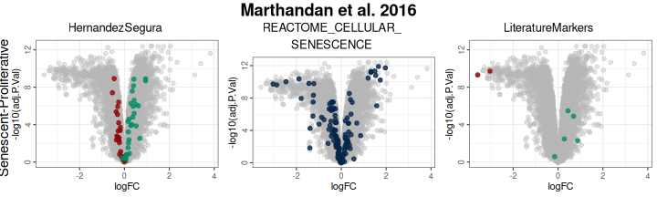
We next apply GSEA to the differential expression results. This evaluates whether genes from each set are non-randomly concentrated at the top or bottom of the ranked list. Results are reported as NES with multiple-testing adjusted p-values. Gene ranking can be based on alternative statistics (e.g., moderated t or B-statistic), which influence whether results are interpreted as enrichment/depletion or as altered directionality. For a full example and explanation, see the online tutorial here.
GSEAresults <- runGSEA(DEGList = DEGs,
                       gene_sets = genesets_example,
                       stat = NULL,
                       ContrastCorrection = FALSE)

GSEAresults
## $`Senescent-Proliferative`
## pathway pval padj log2err ES
## <char> <num> <num> <num> <num>
## 1: HernandezSegura 9.855198e-10 2.956560e-09 0.7881868 0.6263554
## 2: REACTOME_CELLULAR_SENESCENCE 1.575684e-02 2.363525e-02 0.1151671 0.3687291
## 3: LiteratureMarkers 2.571070e-02 2.571070e-02 0.1295475 0.6948631
## NES size leadingEdge stat_used
## <num> <int> <list> <char>
## 1: 2.639527 52 CNTLN,DYNLT3,SLC10A3,CCND1,TOLLIP,DDA1,...[37] t
## 2: 1.450469 128 H1-2,H2BC4,H2BC5,H4C15,IGFBP7,H2BC12,...[31] B
## 3: 1.648483 7 LMNB1,MKI67,GLB1,CDKN1A,CDKN2A,CCL2 tEnrichment curves from fgsea show the running enrichment
score across the ranked list, indicating the distribution of set members
therein.
plotGSEAenrichment(GSEA_results=GSEAresults,
                   DEGList=DEGs,
                   gene_sets=genesets_example,
widthTitle=40, grid = TRUE, titlesize = 10, nrow=1, ncol=3) 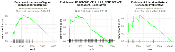
Enrichment results can also be summarised with a lollipop plot, which
compactly shows the NES and highlights statistically significant gene
sets. Here, we can see that the HernandezSegura gene set clearly
exhibits the strongest enrichment signal. When many gene sets and
contrasts are evaluated (which is not the case in this vignette), NES
and adjusted p-values can be summarized in a scatter (volcano-style)
plot for a simpler visualisation, using
plotCombinedGSEA.
plotNESlollipop(GSEA_results=GSEAresults,
                saturation_value=NULL,
                nonsignif_color = "#F4F4F4",
                signif_color = "red",
                sig_threshold = 0.05,
                grid = FALSE,
                nrow = NULL, ncol = NULL,
                widthlabels=13,
                title=NULL, titlesize=12)
## $`Senescent-Proliferative`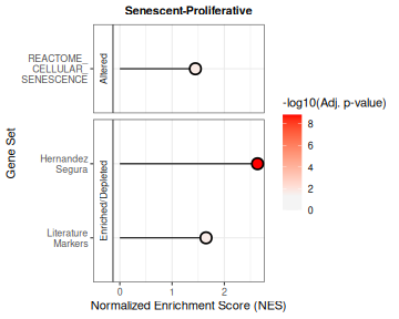
From this exercise in Benchmarking Mode, we can see that two gene sets clearly perform best at discriminating between Senescent and Proliferative conditions: HernandezSegura and LiteratureMarkers. The REACTOME_CELLULAR_SENESCENCE gene set does not show a strong signal; the absense of information on putative gene up- or downregulation upon phenotype potentially dilutes the signal, highlighting the importance of providing directionality when available.
Scoring and enrichment approaches provide complementary insights. Score-based methods offer sample-level resolution, capturing strong contributions from individual genes, while enrichment-based methods evaluate coordinated behaviour across the set.
Discovery Mode
In Discovery (full tutorial here), analyses focus on a single gene set of interest, providing a targeted view of its behaviour across experimental variables (i.e., phenotypes). The output includes:
- Score distributions stratified by variable;
- Effect sizes for pairwise and multiple-group differences (Cohen’s d and f, respectively);
- Cross-variable summaries of NES and adjusted p-values (e.g., lollipop plots).
We illustrate this using the HernandezSegura gene set from our example collection:
HernandezSegura_GeneSet <- list(HernandezSegura=genesets_example$HernandezSegura) For illustration purposes, two synthetic variables were added to the data:
-
DaysToSequencing, the number of days between sample preparation and sequencing; -
Researcher, identifying the person who processed each sample.
This enables exploration of associations between gene set activity and both categorical and continuous variables.
data(metadata_example)
set.seed("123456")
metadata_example$Researcher <- sample(c("John","Ana","Francisca"),39, replace = TRUE)
metadata_example$DaysToSequencing <- sample(c(1:20),39, replace = TRUE)
head(metadata_example)
## sampleID DatasetID CellType Condition SenescentType
## 252 SRR1660534 Marthandan2016 Fibroblast Senescent Telomere shortening
## 253 SRR1660535 Marthandan2016 Fibroblast Senescent Telomere shortening
## 254 SRR1660536 Marthandan2016 Fibroblast Senescent Telomere shortening
## 255 SRR1660537 Marthandan2016 Fibroblast Proliferative none
## 256 SRR1660538 Marthandan2016 Fibroblast Proliferative none
## 257 SRR1660539 Marthandan2016 Fibroblast Proliferative none
## Treatment Researcher DaysToSequencing
## 252 PD72 (Replicative senescence) Ana 6
## 253 PD72 (Replicative senescence) Ana 18
## 254 PD72 (Replicative senescence) John 19
## 255 young Ana 2
## 256 young Francisca 9
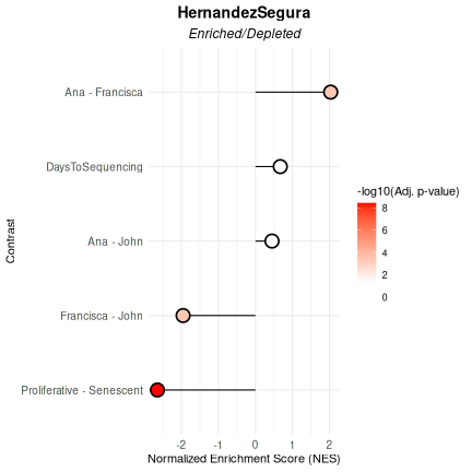
## 257 young John 10We can then examine how the gene set associates with these variables
using enrichment-based approaches in Discovery Mode. The resulting plot
highlights significant associations across variables and visually
summarises the direction and strength of the effects. The “simple” mode
provides comparison of effect sizes across pairwise contrasts between
only two levels of the variable, but can be changed to more levels of
comparison (see ?VariableAssociation).
In this example, the HernandezSegura gene set shows significant enrichment in samples sequenced by Francisca relative to those processed by Ana or John, which would suggest a differentiated researcher-associated technical impact on the samples’ biological phenotype. This gene set shows also a strong depletion in proliferative samples, which is expected given its annotation as senescence-associated and results from the Benchmarking Mode.
VariableAssociation(
  data = counts_example,
  metadata = metadata_example,
  method = "GSEA",
  cols = c("Condition","Researcher","DaysToSequencing"),
  mode = "simple",
  gene_set = HernandezSegura_GeneSet,
  saturation_value = NULL,
  nonsignif_color = "white",
  signif_color = "red",
  sig_threshold = 0.05,
  widthlabels = 30,
  labsize = 10,
  titlesize = 14,
  pointSize = 5
) $plot
Alternatively, score-based methods provide a
per-sample metric of gene set activity, which can then be summarised
across variables. Here, we compute log2-median scores. The
Condition variable shows a large effect size (Cohen’s f),
confirming strong discrimination between Senescent and Proliferative
samples. In contrast, Researcher does not show a detectable
association, in contrast to enrichment-based results. This divergence
illustrates the value of applying both enrichment- and score-based
approaches in a complementary manner.
VariableAssociation(data = counts_example,
                    metadata = metadata_example,
                    method = "logmedian",
                    cols = c("Condition","Researcher","DaysToSequencing"),
                    gene_set = HernandezSegura_GeneSet,
                    mode="simple",
                    nonsignif_color = "white", signif_color = "red", saturation_value=NULL,sig_threshold = 0.05,
                    widthlabels=30, labsize=10, titlesize=14, pointSize=5, discrete_colors=NULL,
continuous_color = "#8C6D03", color_palette = "Set2")$Overall 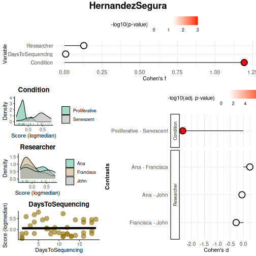
##           Variable    Cohen_f      P_Value
## 1        Condition 1.19407625 1.267423e-08
## 2       Researcher 0.12816159 7.458318e-01
## 3 DaysToSequencing 0.00792836 9.617953e-01
The Benchmarking Mode offers the most comprehensive set of features. Users are allowed to seamlessly move from Discovery to Benchmarking once a variable of interest has been identified and further testing is required. Benchmarking is designed to evaluate multiple gene sets simultaneously, whereas Discovery focuses on the performance of a single gene set.
Individual Gene Exploration
To better understand the contribution of individual genes within a
gene set, and identify whether specific genes drive the set’s collective
signal, markeR provides
VisualiseIndividualGenes. Available options include:
- Expression heatmaps of genes across samples or groups of samples;
- Violin plots showing cross-sample expression distributions of individual genes;
- Heatmaps of pairwise cross-sample expression correlation between genes in the set;
- ROC curves and AUC values to evaluate single genes’ performance as phenotypic markers;
- Effect size estimation (Cohen’s d) of expression differences between groups of samples;
- Principal Component Analysis (PCA) of expression of genes in the set, to evaluate which genes dominate collective variance and how samples separate according to the gene set’s expression.
For a complete overview, see ?VisualiseIndividualGenes
and the extended online tutorial here.
Compare with Reference Gene Sets
markeR also supports comparison of user-defined gene
sets against reference collections (e.g., MSigDB). Two complementary
similarity metrics are implemented:
Jaccard Index: the ratio of the number of genes in common over the total number of genes in the two sets.
Log Odds Ratio (logOR) from Fisher’s exact test of association between gene sets, given a specified gene universe.
Filters can be applied based on similarity thresholds (e.g., minimum Jaccard, OR, or Fisher’s test p-value).
Example of Gene Set Similarity (full tutorial here):
We compare two user-defined gene sets against other user gene set and
the MSigDB C2:CP:KEGG_LEGACY collection. Similarity is summarised in a
heatmap of log odds ratios, highlighting associations above a defined
threshold (e.g., OR > 100 for at least one of the signatures being
compared). The underlying data for the heatmap can be accessed via
$data for further analysis.
# Example data
signature1 <- c("TP53", "BRCA1", "MYC", "EGFR", "CDK2")
signature2 <- c("ATXN2", "FUS", "MTOR", "CASP3")

signature_list <- list(
  "User_Apoptosis" = c("TP53", "CASP3", "BAX"),
  "User_CellCycle" = c("CDK2", "CDK4", "CCNB1", "MYC"),
  "User_DNARepair" = c("BRCA1", "RAD51", "ATM"),
  "User_MTOR" = c("MTOR", "AKT1", "RPS6KB1")
)

geneset_similarity(
  signatures = list(Sig1 = signature1, Sig2 = signature2),
  other_user_signatures = signature_list,
  collection = "C2",
  subcollection = "CP:KEGG_LEGACY",
  metric = "odds_ratio",
  # Define gene universe (e.g., genes from HPA or your dataset)
  universe = unique(c(
    signature1, signature2,
    unlist(signature_list),
    msigdbr::msigdbr(species = "Homo sapiens", category = "C2")$gene_symbol
  )),
  or_threshold = 100,
  width_text=50,
  pval_threshold = 0.05
)$plot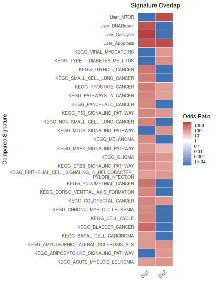
Session Information
## R version 4.6.1 (2026-06-24)
## Platform: x86_64-pc-linux-gnu
## Running under: Ubuntu 24.04.4 LTS
##
## Matrix products: default
## BLAS:   /usr/lib/x86_64-linux-gnu/openblas-pthread/libblas.so.3
## LAPACK: /usr/lib/x86_64-linux-gnu/openblas-pthread/libopenblasp-r0.3.26.so;  LAPACK version 3.12.0
##
## locale:
##  [1] LC_CTYPE=C.UTF-8       LC_NUMERIC=C           LC_TIME=C.UTF-8
##  [4] LC_COLLATE=C.UTF-8     LC_MONETARY=C.UTF-8    LC_MESSAGES=C.UTF-8
##  [7] LC_PAPER=C.UTF-8       LC_NAME=C              LC_ADDRESS=C
## [10] LC_TELEPHONE=C         LC_MEASUREMENT=C.UTF-8 LC_IDENTIFICATION=C
##
## time zone: UTC
## tzcode source: system (glibc)
##
## attached base packages:
## [1] stats     graphics  grDevices utils     datasets  methods   base
##
## other attached packages:
## [1] markeR_1.3.1     BiocStyle_2.40.0
##
## loaded via a namespace (and not attached):
##   [1] pROC_1.19.0.1         gridExtra_2.3.1       rlang_1.3.0
##   [4] magrittr_2.0.5        clue_0.3-68           GetoptLong_1.1.1
##   [7] msigdbr_26.1.0        otel_0.2.0            matrixStats_1.5.0
##  [10] compiler_4.6.1        mgcv_1.9-4            reshape2_1.4.5
##  [13] png_0.1-9             systemfonts_1.3.2     vctrs_0.7.3
##  [16] stringr_1.6.0         pkgconfig_2.0.3       shape_1.4.6.1
##  [19] crayon_1.5.3          fastmap_1.2.0         backports_1.5.1
##  [22] labeling_0.4.3        effectsize_1.0.3      rmarkdown_2.31
##  [25] ragg_1.5.2            purrr_1.2.2           xfun_0.59
##  [28] cachem_1.1.0          jsonlite_2.0.0        BiocParallel_1.46.0
##  [31] broom_1.0.13          parallel_4.6.1        cluster_2.1.8.2
##  [34] R6_2.6.1              stringi_1.8.7         bslib_0.11.0
##  [37] RColorBrewer_1.1-3    limma_3.68.4          car_3.1-5
##  [40] jquerylib_0.1.4       Rcpp_1.1.2            bookdown_0.47
##  [43] assertthat_0.2.1      iterators_1.0.14      knitr_1.51
##  [46] parameters_0.29.2     IRanges_2.46.0        splines_4.6.1
##  [49] Matrix_1.7-5          tidyselect_1.2.1      abind_1.4-8
##  [52] yaml_2.3.12           doParallel_1.0.17     codetools_0.2-20
##  [55] curl_7.1.0            plyr_1.8.9            lattice_0.22-9
##  [58] tibble_3.3.1          withr_3.0.3           bayestestR_0.18.1
##  [61] S7_0.2.2              evaluate_1.0.5        desc_1.4.3
##  [64] circlize_0.4.18       pillar_1.11.1         BiocManager_1.30.27
##  [67] ggpubr_1.0.0          carData_3.0-6         foreach_1.5.2
##  [70] stats4_4.6.1          insight_1.5.2         generics_0.1.4
##  [73] S4Vectors_0.50.1      ggplot2_4.0.3         scales_1.4.0
##  [76] glue_1.8.1            tools_4.6.1           data.table_1.18.4
##  [79] fgsea_1.38.0          locfit_1.5-9.12       ggsignif_0.6.4
##  [82] babelgene_22.9        fs_2.1.0              fastmatch_1.1-8
##  [85] cowplot_1.2.0         grid_4.6.1            tidyr_1.3.2
##  [88] datawizard_1.3.1      edgeR_4.10.1          colorspace_2.1-2
##  [91] nlme_3.1-169          Formula_1.2-5         cli_3.6.6
##  [94] textshaping_1.0.5     ComplexHeatmap_2.28.0 dplyr_1.2.1
##  [97] gtable_0.3.6          ggh4x_0.3.1           rstatix_1.0.0
## [100] sass_0.4.10           digest_0.6.39         BiocGenerics_0.58.1
## [103] ggrepel_0.9.8         rjson_0.2.23          htmlwidgets_1.6.4
## [106] farver_2.1.2          htmltools_0.5.9       pkgdown_2.2.1
## [109] lifecycle_1.0.5       GlobalOptions_0.1.4   statmod_1.5.2